Chapter 2: Heat flow in welding

 

Chapter 2: Heat flow in welding

Temperature Distribution in Welding

Temperature distribution in welding depends upon the nature of the welding process used, type of the heat source employed, energy input per unit time, configuration of the joint (linear or circular), type of joint (butt, fillet, et.c.),physical properties of the metal being welded, and the nature of the surrounding medium i.e. ordinary atmospheric conditions or underwater. Although it is beyond the scope of this book to analyse all these aspects of heat flow in detail but brief descriptions of the following cases are

(A) Arc Welding

(i) Linear butt welds,

(ii) Circular butt welds,

(iii) Fillet welds.

B) Resistance .Welding

(i) Upset butt welding,

(ii) Spot welding.

(C) Electroslag Welding,

(D) Underwater Welding.

Temperature Distribution in Arc Welding

Nearly 90% of welding in world is carried out by one or the other arc welding process, therefore it is imperative to discuss the problem of temperature distribution in arc welding in the maximum possible detail to arrive at the best possible understanding of the problem. Because linear butt welds are perhaps the most used type of welds in welded fabrication therefore this type of joint will be detailed the most.

Temperature Distribution in Linear Butt Welds

Heat flow in welding is mainly due to the heat input by wetding source in a limited zone, and its subsequent flow into the body of the workpiece by conduction. Alimited amount of heat loss is by way of convection and radiation as well but that can be accounted for by allotting heat transfer efficiency factor at the accounting of heat input. So, the problem of temperature distribution can be seen as a case of heat flow by conduction when the heat input is by a moving heat source. This case can be further simplified by assuming workpiece of large dimensions to approach the infinity concept i.e. the temperature at the farthest end of the workpiece in all directions remains unchanged', This leads to a condition of quasi-stationary state which can be defined as a condition in which an observer at the arc will see a fixed temperature field all around the arc at all times. In other words under a condition of quasi-stationary state of heat flow isotherms representing, different temperatures remain at a fixed distance with respect to the heat source. Mathematically stated it means dT/dt = 0 

where T is the temperature at any time and t is the time unit. Fig. 2.1 represents the condition of quasi-stationary state with observation points at A and B for welding along centre line of the plate. To determine the temperature at any point, in a workpiece, during welding, the problem can be solved by considering from the basic Fourier's Equation of heat flow by conduction,

If one dimensional form of heat conduction is considered as shown in Fig. 2.2, Fourier's Law states that the rate of heat transfer per unit time, q, is a product of,

(a) area, A, normal to heat flow path,

(b)the temperature gradient at the section i.e. the rate of change of temperature with reference to the distance in the direction of heat flow,

(c) k, thermal conductivity of the material of the body.

Mathematically stated,

where, dQ = quantity of heat conducted in time, dt .

Note: (i) Since the heat flow always occurs in the direction of decreasing temperature, the temperature gradient (dt/dx) will,therefore, always be -ve, hence the negative sign on the right hand side of the equation (2.1).

(ii) The following assumptions have been made in the above equation,

(a) the heat flow in y and z directions is zero,

(b) the temperature in any plane perpendicular to the x-axis is uniform throughout the plane.

The equation (2.1) represents the fundamental heat conduction law for uni-directional flow of heat. As normally the heat will flow in all the three directions in a given body, therefore a comprehensive equation must deal with 3-dimensional heat flow. Three Dimensional Heat Flow Equation

Consider an infinitely small solid cubic body as shown in Fig.2.3.

Let the edges parallel to the three axes be respectivelydx, dy and dz. The volume ofthe cubicelement is, therefore, given by the relation,

Let dQx represent the total quantity of heat entering the face area dy . dz in time dt as shown in Fig. 2.3. So, on the basis of equation (2.1), we have,

Note: The gradient in equation (2.3) is expressed as a partIal derivative of the temperature T as it is a function of x, y, z and t. Now,a corresponding quantity of heat will be leaving the cubic element (dx . dy . dz). Let it be dQx + dx, the value of which may be obtained by Taylor Expansion of dQx + dx' whereby,

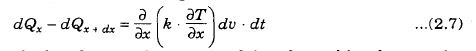
Ignoring the higher terms of Taylor expansion in equation (2.4), the net heat gained by the element (dx· dy . dz) due to conduction in x-direction will, thus, be,

By substituting the value of dQx from (2.3) in the right hand side of equation (2.5), we get,

From (2.6) and (2.2), we get,

Similarly, the net heat gained by the cubic element by conduction in y and z directions may be obtained as follows,

The total heat gained (dQ) by the cubic element (dx . dy . dz) is the sum of the heat gained by conduction in x, y, and z direction. Thus, from equations (2.7), (2.8) and (2.9), we get,

Now, the heat gained by the cubic element (dx . dy . dz) can also be expressed in terms of increase in internal energy dE, expressed as,

Assuming k uniform in all directions of the equation (2.12) can be written as,

where (α) is known as the thermal diffusivity of the material of cubic element and its unit is m2/sec.

From equations (2.13) and (2.14), we get,

This is known as Fourier's Equation of three dimensional heat conduction in solids. To apply equation (2.15) to welding, let us consider the situation in arc welding as expressed in Fig. 2.4.

Let 0 be the origin (i.e. the starting point for welding) for the cartesian coordinates (x, y, z). Suppose, we are interested in finding temperature at any point A (x, y, z). Because of moving heat source the distance of point Ais changing every moment with respect to the arc or the tip of the electrode. If the origin of coordinate system is shifted from 0 to the tip of the electrode (which is assumed to lie in the plane of top surface of the plate) then the temperature at any point A located at a fixed distancE)from the tip of the electrode remains fixed because of the establishment of a quasi-stationary state and can thus be determined mathematically.

Let point A in the new coordinate system with respect to the tip of the electrode have the coordinates

where, v = the welding speed,

t = time taken by welding, starting from the origin, O.

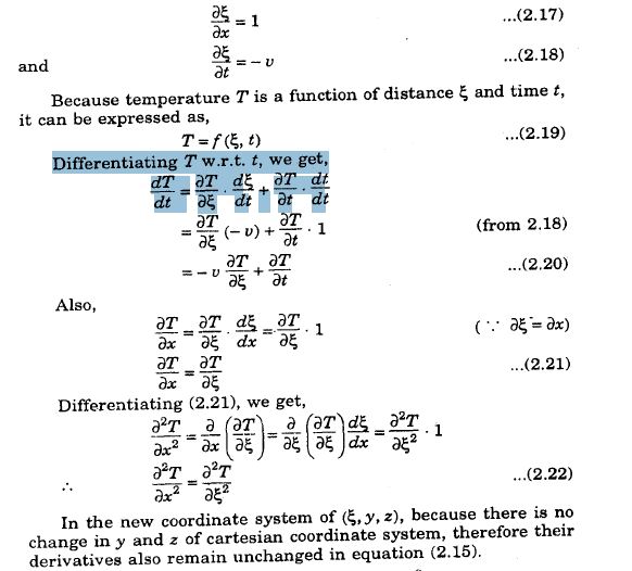
Now, to determine the temperature distribution in the plate with respect to the tip of the electrode, we are required to change equation (2.15) from cartesian coordinate system (x, y, z) to a new coordinate system

Differentiating (2.16), we get,

Equation (2.32) is a more convenient form of heat flow equation for a quasi-stationary state of welding. It can be used for determining temperature distribution in specific cases for example, in a semi-infinite plate which is representative of welding a large thick plate.

Temperature Distribution in a Semi-Infinite Plate (3- dimensional case)

Considering a case of laying a single weld bead, using a point heat source, on the surface of a very large and thick plate (workpiece), as shown in Fig. 2.5. Let us assume that the Z-axis is placed in the direction of thickness of the plate downwards. For determining the temperature distribution the solution of equation (2.32) must satisfy the following conditions.

(1) Since welding is done by a point heat source, the heat flux through the surface of the hemisphere drawn around the source must tend to the value of the total heat,Qp delivered to the plate, as the radius of the sphere tends to zero. If R is the radius of the sphere, then the total heat flowing through the hemispherical surface of heat source as given by Fourier's Equation will be,

(2) Heat losses through the surface of the plate (workpiece) being negligible, there is no heat ransmission from the plate to the surroundings

(3) The temperature of the plate remains unchanged at a great distance from the heat source

Now, condition (2) i.e. equation (2.36) assigns a semi-circular form to the isothermf: located at sections parallel to plane YZ (Fig. 2.5), thus they are dependent only on radial distance 'l' from the heat source. Keeping in view the semi-circular form of isotherms, equation (2.32) can be written more conveniently in cylindrical coordinates, as shown in Fig. 2.6.

Now, temperature Φ is a function of y and z while y and z are functions of l and therefore equation (2.32) can be converted into polar coordinates by determining the double differential of  Φ w.r.t. and z in terms of Z and 

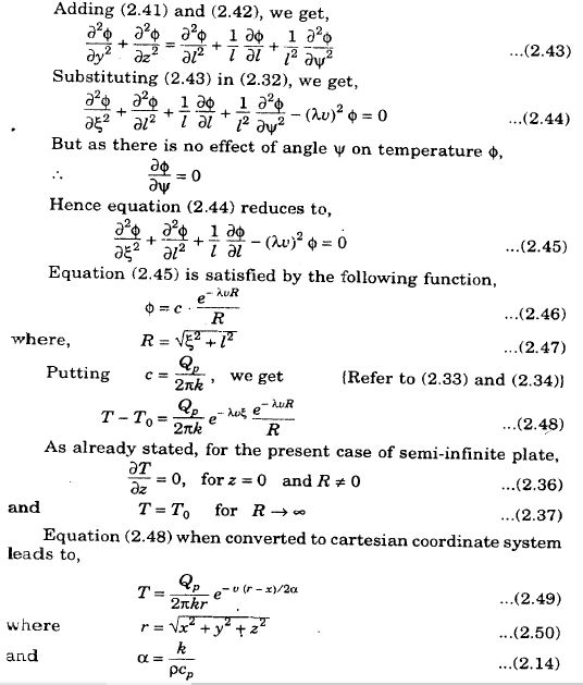
Equations (2.48) and (2.49) are important relationships for determining temperature distribution in a semi-infinite plate.

2.1.1.3 temperature distribution in large (infinite) plate of finite thicknes

Equation (2.48) can help in determining temperature distribution in semi-infinite plate but the normal cases encountered are those of large plates (in ship-building and pressure vessel fabrication, etc.) of finite thickness. Thus, equation (2.48) must be modified to account for the limited range of Z dimension.

Therefore, boundary condition of equation (2.51) is satisfied. However, it. remains to be proved that conditions of equations (2.33) and (2.35), viz.,

Equation (2.62) satisfies equations (2.33) and (2.35).

To sum up it can be said that the following two equations can be used for determining temperature distribution during butt weLding of large (semi-infinite) plates of infinite thickness and finite thickness respectively .

2.2. Efficiency of Heat Sources

It is evident from the solution of Problem 2.1 that to solve the temperature distribution problems we require to know the efficiency η  of the heat source used for welding ; where η defined as,

Thus, if the efficiency η of the heat source is known, the energy (Q) transferred from it to the workpiece, can be determined. In arc, electroslag, and electron beam welding,

where V and I are the arc voltage and welding current respectively. In gas tungsten arc welding (GTAW)with dcen (direct current, electrode negative) the majority of the heat is produced by electrons bombarding the workpiece (anode) that is as a result of the release ofthe work function and the conversion oftheir kinetic energy into heat at the workpiece. In GTAWwith a.c., however, electrons bombard the workpiece only during straight polarity half cycle i.e. for a period when electrode is negative thus resulting in significantly lower arc efficiency. Also, the heat loss to the surrounding can be rather high; particularly so for long arc lengths. Apart of the heat generated is taken away by the cooling water employed to keep the electrode cool. In consumable electrode welding processes like SMAW,SAW, GMAWand FCAW,using dcep or a.c. the heat going to both the electrode and the workpiece finally lands up on the workpiece through transfer of molten meta1. Thus, the heat transfer

efficiencies of these processes are high. In SAW process, the heat transfer 11 is further increased because the arc remains under a blanket of flux, the heat loss to the surroundings is, thus, minimised.

The efficiency of heat transfer in ESW is lower than that in SAW, mainly owing to heat loss to the water-cooled copper shoes and, to lesser extent, by radiation and convection from the surface of the molten slag.

the molten slag.

In EBW (electron beam welding) process the welds are produced by the phenomenon of keyholing. These keyholes act like bIack bodies to the heat source and trap most of its energy; leading to very high efficiency of heat transfer in EBW process.

In laser welding the heat transfer efficiency can be strongly affected by the wavelength and energy density of the laser beam, the workpiece material and its surface condition, and the joint design. For example, with well poli>Shed AI or Cu, the surface reflectivity can be around 99%, i.e. the efficiency can be only about 1% for a 10.6  μm.continuous wave CO2 laser. For steels, especially when coated with thin layers of materials that enhance absorption of the beam energy (for example, graphite and zinc phosphate), quite reasonable efficiencies can be obtained. When keyholes are established during laser welding, the efficiency of the process can rather be impressive.

In Oxy-acetylence welding the energy transferred is given by,

Both these values refer to standard state of 1atm, and 25°C tem perature.The heat source efficiency in Oxy-acetylene gas welding varies over a rather wide range as the efficiency decreases significantly

with increasing fuel consumption rate VC2H2 , because of incomplete 2 ·2 combustion. Efficiency of oxy-acetylene gas welding is also found to depend on the torch nozzle diameter, welding speed, material thickness, and thermal conductivity of the workpiece. In Table 2.1 are listed the efficiencies of most of arc. beam and flame welding

2.3. Further Modifications of Temperature Distribution Equtions

Different researchers have tried to modify Rosenthal's equations to determine more accurately the temperature distribution under different sets of welding conditions. The ones put forward by Adams, and Wells have received wide recognition and are included in the following sub-sections.

2.3.1. Adams Modification

In the earlier treatment of problem based on Rosenthal's solution the heat source has been assumed to be a point heat source which is obviously not true, particularly for small sized workpieces. Thus, recognising the existence of finite sized weld pools, Adams used the fusion line as the boundary condition and modified Rosenthal's equations viz., equations (2.48) and (2.62). The following equations were derived by Adams for the peak temperature, Tp, at a distance y from the fusion boundary at the workpiece surface.

2.3.2. Wells Modification

The relationship between the heat flow and weld bead dimensions is given by the Wells simplification of Rosenthal's Equation by the following relationship.

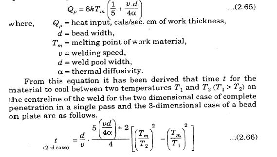
The main difficulty in the use of heat flow equations is the variation of physical constants (like k, p, C, etc.) with temperature. Energy absorption within the weld pool by latent heat and its subsequent release at the tail end of the weld pool on solidification is one reason why actual isotherms around a moving weld pool are more elongated than indicated by calculations. Wells equations (2.65) to (2.67) give good corr~lation with experimental data for low carbon steel and can be adjusted to apply more accurately to

metals having high latent heats by using.a specific heat value corrected by the following relationship.

Heat Flow in Fillet Welds

A simple approach to analyse heat flow in T-type fillet welds is to assume that the total heat supplied from the arc is distributed in the three plates in the ratio of their thicknesses. Temperature distribution in the three plates forming the fillet joint can then be determined individually with the help of formulas used for determining temperature distribution for laying bead-an-plate on moderately thick plates i.e. equation (2.62). This approach implies that if three plates have equal thicknesses, temperatures at points equi-distant from the centre of the weld should be same in the three plates. This, however, does not hold good at early stages of heat flow from the weld centre though all three heat distributions approach similarity as the time passes. This leads to a conclusionthat the bead-an-plate analysis can be applied successfully to fillet welds for determining temperature distribution except 

(i) at the early stages of welding, and

 (ii) 0 the points close to the arc. 

The deviation is large when the arc is passing just over the point under consideration. However, it decreases and ultimately the temperature distributions show no differences as the time passes, as shown in Fig. 2.8. Such a deviation at earlier stages of welding a fillet joint can be accommodated by introducing a factor which approaches unity with time. If equation (2.62) is multiplied by this factor, the temperature deviations at earlier stages can be duly accounted for finding the true temperature distribution in fillet welds. For this purpose an exponentially varying factor ofthe form 

 is considered most appropriate where A and B are constants, the magnitudes of which depend upon the thickness ratios of,three plates, etc. If equation (2.62) is expressed in a simple form as,

(where b stands for bead-on-plate welds) then the modified relationship is obtained by multiplying equation (2.73) by a factor mentioned above. Thus, for fillet welds the temperature distributi. on can be expressed as,

where f stands for fillet welds.

GuptTahearvea,lues of the constants A and B as reported by Gupta and

A = 0.598 and B =0.029

It is further reported by the same authors that in T-type fillet welds the vertical plate shares the maximum instantaneous heat while the back portion of the flange, that is the one opposite to where the weld is laid shares the least amount of heat. This condition makes fillet welds susceptible to high degree of distorticill and non-uniform metallurgical changes compared to butt welded joints.

Heat Flow in Circular Welds

The highest strain in welded structures form after making welds that do not finish on the free edges of the workpiece. This includes a large group of circular welded joints i.e. the welding of various types of patches, flanges, nipples, connecting pipes and many other cylindrical components. The strains in such welds may be considerably reduced by altering the design of the weld and the fabrication technology employed. To do so, it is imperative to evaluate the temperature field formed in the component during

welding, and to select correctly the optimum parameters that control this field.

Considering the temperature dependence of the thermophysical properties of the material i.e

and the heat transfer from the surfaces of the workpiece, the volume nonequilibrium distribution of heat in workpiece in the welding of circular joints is described in the cylindrical system of coordinates 

by the following equation,

Considering specific cases of automatic welding of circular joints with a radius of 15 em in 8 mm thick plates of AlMg6 alloy at a speed of 36 m/hr (1 em/see) under three different heat transfer' conditions, viz.,

(i) welding without any backing plate,

(ii) welding with a backing plate of steel,

(iii) welding with the lower surface of the plate water cooled

The coefficient of heat transfer at the bottom of the plate for the above three conditions were taken respectively as 2.092 x 10-3, 20.92 X 10-3 and 209.2 x 10-3W/cm2_oC.

Welding was done in a single pass with a 2 mm diameter wire using a welding current of 308 A with dcep polarity at an arc voltage of25 V and a wire feed rate of 500 m/hr (8.33 m/min). The temperature distribution patterns obtain,ed respectively for the three cases were reported to be as shown---inFigs. 2.9, 2.10 and 2.11. Fig. 2.9 shows the temperature field in sections 1-3 and 2-4. Jt is seen that in the case of heat transfer from both sides of the plate to the ambient air central part of the plate is heated to high temperatures. In the course of welding, the heat source moves over th e already heated zone resulting in increased dimensions of the cwirecllde. pool and that displaces the pool towards the centre of the circle

Fig. 2.10 shows the temperature di.stribution when AI-alloy plate is resting on a steel plate during welding. It is evident that the temperatures are all along reduced, as compared with the first case, indicating a higher heat sink effect provided by the steel backing plate. Fig. 2.11 shows the temperature distributiun when the AIMg6 plate is water-cooled at the bottom. It is evident that in this case the source moving along a circle may be replaced by a circular source applied to the entire circumference of a circle with radius "0. however this substitution cannot be applied to earlier two cases. In practice, the concept of a circular heat source may be used with success in calculation of temperature fields in certain specific cases. These cases include the heating of a sheet surface with a rapidly moving electron beam, with high frequency induction coils, the resistance welding of nipples, GMAW at speeds above 60 m/hr, etc. Taking the above considerations into account temperature distribution under the effect of a circular source can be devived. The differential equation of heat conduction for this case has the

following form :

Fig. 2.12 shows the temperature field in the welding of 8 mm thick plate with the circular heat source and without any backing strip. The calculated results given in. Fig 2.12 are based on equation~ (2.76) and (2.88). This figure indicates that at high temperatures the data calculated with and without the consideration of the effect of temperature on thermophysical properties have considerable differences.

For calculations in the above mentioned cases the AlMg6 plates were considered with the values of different parameters as given below.

Heat Flow in Resis~ance Welding

In this section two types of resisting welding processes viz., spot welding and zonetl w~lding are discussed. The discussion will be confined to resistance 'l'lpotwelding and upset butt welding to represent the two types of welding processes.

Heat Flow in Resistance Spot Welding

There are three important variables in resistance spot welding VlZ. , current, time, and pressure. In any resistance welding process the heat generated by the passage of current is given by either of the following two equations.

Current, voltage, and resistance all vary with time.

Of the total heat generated i.e. Q, only a fraction is used to make the weld. The balance leaks into the work, and more so to the water-cooled copper alloy electrodes of high electrical and thermal conductivities. It is obvious that, for a given quantity of heat generated (Q), the longer the time of generation, the larger the fraction that leaks off. Further, it can be shown mathematically that the rate at which the heat leaks away from the weld is a maximum at the beginning of the weld period (because of cold workpiece) and that the amount of heat loss is proportional to the square root of the duration of the weld time.

If heat transfer efficiency be taken as the ratio of the volume of steel actually melted by a fixed quantity of heat to the volume which could be melted if no heat were lost then the weld time versus efficiency curvefor Q = 300 cals is shown in Fig. 2.13. This curve is plotted for a theoretical spot weld made by generating heat at a point source between two steel sheets in contact. It can be seen from this figure that the maximum possible efficiency obtained, when the heat is generated instantaneously, is 60%. For 300 calories generated in 1 see, the efficiency is only 1%. For a typical spot welding operation, 3000 calories per second for 0.1 see, the efficiency is about 10%. Thus, it is evident that for resistance spot welding as well as for other similar processes, for example, seam welding, projection welding, etc., these must be inherently short time, high current processes. Most of the features of these processes, and many of the industrial problems met with in their applications, are caused by this limitation.

Considering the case of resistance spot welding, let Q calories of heat be generated instantaneously at a point within an infinite body. The temperature distribution about the point, as a function of time and distance is given by,

Thus, for a given amount of heat input, the peak temperature at any point is inversely proportional to the cube of the distance of this point from the point at which the heat is introduced. Putting T=1500°C, Q=.300 calories, C=0.12 cal/gm.°C, ρ = 7.8 g/cm , we get, r = 0.25 cm.

This locates t = 0 point for the curve of Fig 2.13. Weld time versus efficiency of heat utilisation in spot, seam, and projection welding is given by the inset curve in Fig. 2.13. It is evident that the weld time duration should approach as Iowa value as possible.

It is therefore imperative to use very high welding current in all these resistance welding processes.

Heat Flow in Upset Butt Welding

In general the welding processes require that a certain temperature be reached and maintained long enough for the weld to be completed. For example, in upset or resistance butt welding the aim is for an interface temperature of the order of the solidus temperature, Ts, of the work material. This temperature when reached needs to be held only until the oxide layer at the interface has been dislodged by fragmentation or diffusion, or until sufficient lengths of the workpieces have been heated to permit upsetting.

Let us consider upset butt welding of two round bars of steel, each of length l and cross-sectional area A. Assume that the interface is raised instantaneously to the solidus temperature, Ts, and that the opposite ends of bars are held at room temperature. To determine the temperature variation, along the length of the bar, with time let us consider an element of thickness dx of the bar centred x cm from the interface as shown in Fig. 2.14.

Assume that the interface has been at temperature Ts long enough so that the element has a temperature above the room temperature, To: but has not attained as yet its steady-state temperature.

The partial derivate indicates that the heat flow at a definite time t is being considered. At face I of the element, heat is flowing at the rate ql as given by the following equation,

where the second derivative indicates that there may be a change in gradient as we move from plane x to the boundary plane I. Similarly at face II, we have,

If surface losses are neglected, the difference qI - qII == qn gives the rate at which the heat is accumulating in the element,

Now, if the heat is accumulating in the differential element, its temperature must be changing. Taking c as the specific heat of bar material and p its density, and assuming that these also.do not change with temperature T, thus qn can also be given by the following relationship,

where refers to the rate of change of temperature on the plane x. Equating the right hand sides of equations (2.102) and (2.101), we get,

Equation (2.103) is a general equation for any case of unidirectional heat flow through a body containing no heat source(s) and no heat sink(s) other than its own heat capacity. \Vhen extended to three dimensional heat flow system it reads as

Now,to solve the differential equation (2.103) \ye must find a solution that satisfies the following boundary conditions.

It is also known from steady-steady-state heat conduction theory that when t =∞ the solution ofequation (2.103) must reduce to,

The most general solution to equation (2.104) for the period representing the interval before any heat has reached the ends of the bars is a temperature distribution given by,

(erf u) can be obtained from standard mathematical tables. Equation (2.106) fails if it indicates that the temperature at ± l is increasing. Thus, to test the valadity ofa temperature distribution obtained by its use, it is merely necessary to calculate e at x = l at the desired time. If et is greater than 5 or 10 degrees (above the ambient), the distribution will be inaccurate. Fig 2.15 illustrates

the application of this equation for l == 10 cm for the aforementioned boundary conditions. The actual temperature distribution generally looks more like the dotted curve of Fig. 2.15.

Heat Flow in Electroslag Welding

In electro slag welding (ESW) the heat source is large and moves slowly. This implies that the material ahead of the moving heat Source is preheated to a much higher degree than in normal arc welding so that the heat flow patterns associated with ESW are not likely to be well described by considering point heat source. Also, the important role of the slag in this process with its resistive heating effect should also be taken into account particularly with regard to its effects on the shape and size of the heat Source. Because the slag volume is quite large in ESW thus the assumption of a point heat source is not representative of this Attempts to simulate. the heat flow of ESW have been made by different researchers. One such model based on symmetrical parabolic model to represent the moving molten-solid interface yielded fairly satisfactory results typical isotherm shapes as calculated from such a model are shown in Fig. 2.16.

Heat Flow in Underwater Welding

The process of underwater welding is broadly divided into two types viz., Dry Underwater Welding, and Wet Underwater Welding. In dry underwater welding the spot to be welded is enclosed by a chamber from which water is excluded under pressure. The welding so done is very similar to that carried out in open air conditions except that the pressure varies with the water depth. Temperature distribution in the work therefore remains similar to that encountered in normal atmospheric welding.

Wet underwater welding is carried out in water without any chamber around the spot to be welded. The process basically remains same as used in normal open air welding but the change from air to water environment results in higher heat losses and the arc is constricted. In wet underwater welding the heat losses from the surface of the workpiece are so high that the temperature at a short distance from the outer periphery of the weld pool remains unaltered which results in the establishment of very

steep thermal gradients. Thus, the isotherms are confined to a very narrow zone which makes experimental measurements of temperature, at a point, quite difficult. The present discussion about heat flow in underwater welding is limited to wet underwater welding only.

Heat Flow in Wet Underwater Welding

In wet underwater welding the heat flow takes place inside the workpiece by conduction while heat flow by convection accounts for most of the heat dissipation from the surface of the workpiece. The temperature distribution inside the solid body, away from the heat source, is very well accounted for by Fourier's 3-dimensional, heat flow equation (2.15) and by differential equation of the quasi-stationary state of welding, that is, by equation (2.26) ; however the heat transfer at the surface of the

workpiece is by convection. At the two major bounding surfaces, since the heat is transferred through the laminar boundary layer of fluid only by conduction, thus at these surfaces equation (2.15) reduces to,

This transfer of heat from the surface of the workpiece could also be represented by Newton's law of cooling as,

Equating the right hand sides of equations (2.107) and (2.108), we get,

Fig 2.17 shows that equation (2.109) is valid only for z=0, whereas at z = g, expressicns (2.107) and (2.108) lead to,

Fig. 2.17. Plate with equidistance grid spacing and the direction of outwardly drawn normal at one of the grid points

or, in general, the bound'ary conditions at the two major bounding surfaces could be expressed as,

The quenching caused by the surrounding water in wet underwater welding results as, already discu"ssed, in the setting up of steep temperature gradients in the body of the workpiece. Therefore, the temperature of the plate drops to ambient comparatively at a short distance from the weld pool. Hence, it is logical to assume that the temperature at the periphery of the workpiece must be the same as that of the surrounding water. A solution of temperature distribution problem for wet underwater welding would be one that satisfies simultaneously equations (2.26) and (2.111). To achieve this the values of a (thermal diffusivity), k (thermal conductivity), and h (surface heat transfer coefficient) must be known. Though it is possible to use some average values for a and k without any serious effects on the final results but the change in the value of h with temperature is so large, over the temperature range encountered in welding, that to assume any single value for it is out of question. To arrive at any conclusion about the value(s) ofh to be used a thorough insight into the effects of different situations developed in wet underwater welding on this parameter is required and the same is done in the following sections.

Surface Heat Transfer Coefficient

In underwater SMAWthe arc is surrounded by a very active vapour pocket which dissociates 12 to 16 times per second from around the arc. This keeps the water in the vicinity of the arc always in an agitated state. Thus, it is not the case of what is termed as 'pool boiling' in which the whole volume of the water involved boils and thus stirs without agitation due to any external source.

The value of the surface heat transfer coefficient, h, depends upon the temperature difference between the workpiece and that of the surrounding water as has been expressed by equation (2.108) and the temperature of the work (steel) may vary from around 2500°0 to the ambient water temperature. Moreover due to the very high temperature of the arc the water immediately around the vapour pocket boils. Owing to the agitation of water and convection currents the boiling water moves up, comes in contact with the bulk and gets condensed. Thus, the heat transfer around the arc and consequently the weld pool is high and a very complex phenomenon involving heat transfer by conduction, convection and radiation. The convective heat transfer is further complicated because it involves simultaneously the phenomenon of boiling and condensation. Boiling heat transfer is itself quite complex because apart from the phase change it involves a large number of variables such as the geometry of the work, the viscosity, density, thermal conductivity, expansion coefficient, specific heat of the fluid, the surface characteristics, surface tension, latent heat of evaporation, liquid pressure, etc. Moreover, in underwater welding it is not a case of pool boiling but instead it is a case of what is known as 'Local Boiling', or 'Surface Boiling', or more comprehensively termed as 'Surface Boiling of Subcooled Liquid'. Before discussing 'Local Boiling' a note on the mechanism of 'Pool Boiling' is imperative as that forms the basis to which all deviations will be referred to. 

Pool Boiling

Consider a heated plate submerged in a pool of water at saturation temperature (Tsrd)' As the temperature of the work (Tsat) is raised the value of the heat transfer coefficient, h, goes on increasing. Fig 2.18 represents the type of heat transfer data obtained as the work temperature is increased above ambient. In t.his figure heat flux (q/A ) and surface heat transfer coefficient, h, are plotted against the excess temperature ▲T, where

▲T = Tw - Tsat

As the temperature Tw is raised, ▲T is increased, convection currents cause the liquid to circulate and the steam is produced by evaporation at the liquid surface. This is represented as regime 1 ann is called 'Interface Evaporation'. Here, only the liquid is in contact with the heated surface and the heat transfer is due only to free convection.

With further increase in Δ T the energy level of the liquid adjacent to the work surf~ce becomes high at a number offavoured spots where vapour bubbles are formed. They rise above the plate 8m-face but condense before reaching the liquid surface. This is known as regime 2. As the temperature of the work is raised further, up to point A in the figure, the bubbles become more numerous. The liquid is so hot as not to allow any condensation of the bubbles which rise to the free liquid surface and help rapid evaporation. This is known as regime 3. Both the regimes 2 and 3 fall in the category of 'Nucleate Boiling'.

Beyond the point A, representing the critical heat flux, the number of bubbles formed is so high that they form patches of vapour film which form and break regularly. This constitutes r.egime 4 and is often termed as 'Unstable Film Boiling'. Any further increase in heat input to the work results in the formation of continuous vapour film over the whole body of the workpiece. This is termed as regime 5 and is called 'Stable Film Boiling'. The regimes 4 and 5 are also often simply termed as 'Film Boiling'. Here the number of bubbles formed is so large that they almost cover the whole of the work surface and provide insulating effect. This counteracts the beneficial effects of agitation by bubbles and results in decrease in the heat flux. The vapour film is unstable in regime 4, as under the action of circulating currents it collapses but reforms rapidly. In regime 5 the vapour film is stable and the heat flow is the lowest. For values of ΔT beyond 550°C (regime 6) the temperature of the work surface is quite high and heat transfer occurs predominantly by radiation, thereby increasing the heat flux.

Local or Surface Boiling

The boiling process in a liquid whose bulk temperature is below the saturation temperature but whose boundary layer is sufficiently superheated that vapours form next to the heated surface is usually called 'Local Boiling'. These vapour bubbles break off and begin to rise through the cooler liquid and get condensed to the liquid phase again. Thus boiling at the heated surface is combined with convection at a distance from it and condensation of vapour at the interface between the boiling boundary layer and mass of cold liquid. The intensity of vaporisation on the wall depends on the degree of superheat of the liquid, the process of condensation is determined by difference between saturation temperature and the bulk temperature, that is by the degree of subcooling of the liquid.

Subcooling from the saturation temperature to the bulk temperature is a reference parameter that distinguishes surface boiling from pool boiling. If superheating determines the intensity of vaporisation, subcooling determines the size of the region that is affected by the disturbing action of vaporisation. The greater the subcooling of the liquid, the narrower is the region where boiling takes place. Also, the bubbles increase in number while their sizes and average life time decreases with decreasing bulk temperature at a given heat flux. As a result of increase in the bubble population, the agitation ofthe liquid caused by the motion of the bubbles is more intense in a subcooled liquid than in a pool of saturated liquid and thus much higher heat flux is attained before any vapour film is formed. To appreciate the effect of subcooling on critical heat flux reference may be made to Kutateladze's equation given below.

Putting the values of different variables for the actual condition of operation, with bulk water temperature of30°C it was found that,

which means that the critical heat flux increased 2.565 times for 70°(; of subcooling.

Apart from subcooling other major factors that affect heat flux, and consequently the surface heat transfer coefficient are the arnbient pressure, position of heated surface and the motion of the fluid. The effects of these factors are discussed as follows.

The effect of Pressure

The effect of pressure on the heat transfer coefficient in well developed nucleate boiling is more or less the same for all liquids. According to test data reported by Mikheyev the peak heat flux  first sharply increases, reaches a certain maximum with rising pressure, then drops to zero at critical pressure. If a graph  then the curve is nat its maximum for If this data is applied to water  it will be seen that the peak occurs at. a pressure equal to 80 atmosphere. Further, it has been recommended, from the charts plotted for pressures ranging from P == 0.2 to P == 100 ata., that the coefficient of heat transfer of water in nucleate boiling may be calculated from the following relationship,
                                          

The relationship suggested by Jackob and Hawkins for finding the effect of pressure on heat transfer coefficient is given by the equation,

where, P = pressure of water at the point under consideration,

The Effect of Position of Heated Surface

The heat transfer coefficient, h, and the heat flux (q/A) depend to a great extent, upon the conditions in which the generated vapours separate from the heated surface. These conditions are most favourable in the case of horizontal heated surfaces, the heated side of the surface facing upwards. The aforementioned equations

to

 hold good for such conditions. If the heated side of the work faces downwards, the conditions in which vapours separate from the surface deteriorate sharply and the peak heat flux diminishes by as much as 40%. This is because the motion of the fluid is only in a thin layer undE;rneath the work, the rest of the fluid below that layer remains stationary. Fig. below represents the commonly accepted nature of convection currents above and below a horizontally placed heated

Fig. below  represents the commonly accepted nature of convection currents above and below a horizontally placed heated flat plate.

The Effect of Motion of Fluid

Apart. from the aforementioned factors, heat transfer coefficient is considerably influenced by the rate of forced circulation of the fluid. If there be no forced circulation of the liquid the steam bubbles which are generated on the heated surface grow to a specific size before detachment thus the heat transfer coefficient isgovemed by the intensity ofvaporisat ion. If the liquid is made to circulate then the steam bubbles are detached before they attain critical size. As the fluid density is increased further the effect of intensity of vaporisation is gradually reduced till it reaches a value that of free convection in a single phase liquid. Thus it can be said that at low circulation velocity (w) the intensity of vaporisation (qv) is predominant and at higher circulation velocity the effect. of 'w' is predominant or in other words the

coefficient of heat transfer can be expressed as,

In the case of underwater SMAW,when an arc is struck between the electrode and the workpiece a bubble or a vapour pocket is formed with the arc at its centre. Next to the arc would probably be a mixture of incandescent gases emitted by the' arc and superheated steam around this an envelope of saturated steam in contact with ambient water. The vapour bubble fluctuates, as stated earlier, 12 to 16 times per second releasing about 200 cm3 of combustion gases and steam per second. This leads to enormous disturbance ofliquid in a sufficiently big volume around the arc.

From the factors discussed above and also because of the wide variations in the results of many researchers in the field of boiling heat transfer it is rather difficult to arrive at any standard relation for predicting boiling heat transfer coefficient for the conditions under consideration. However, from the above considerations the different values of heat transfer coefficient, for different ranges of telnperatures, can be based on the careful study and weightage given to different factors discussed as follows.The peak value of 'h'· for pool 'boiling given by Mikheyev is 5 x 10^4 Kcals/m^2hr-°C, and that by Kutateladze is about 2.55 x 10^4 Kcals/m2-hr-°C. Kutateladze has also recommended equation

(2.112) for finding the effect of subcooling on the value of h. Using this equation with 70°C of subcooling (i.e. for a room temperature of 30°C) h increases, as already stated, by a factor of 2.565 thus

giving peak value of h as 6.3 x 10^4 Kcals/m2-hr-°C. Taking into consideration these two values and the agitational effect of the detaching bubbles around the arc it is considered best to use Mikheyev's expression and the subcooling factor found by equation (2.112) to get peak value of h of the order of 12.8 x 10^4 Kcals/m^2-hr-°C.

The different values of' 'h' for work temperature up to 121.5°C could be decided on the basis of results given by different researchers. However, for work temperature higher than 121.5°C, h can be taken as equivalent to peak value mentioned above because it is not a case of pool boiling and there being considerable disturbance around the arc the application of the formula of continuous film to the work being welded appears to be impractical. Moreover, the use of peak value of h for higher temperatures also takes care of heat transfer by radiation above 550°C.

Thus, from the above mentioned considerations the values of surface heat transfer coefficient, h, for different ranges of temperature, encountered in wet underwater welding may be taken as follows.

(i) Heat transfer coefficient can be taken as directly proportional to the temperature difference between the work and the bulk of water for and up to Tw = Tsat = 100°C.

(ii) For interface evaporation, i.e., for the work temperature between 100.1 and 104.7°C,

h = 896 (▲T)^1/3 x subcoolingfactor" Kcals/m^2-hr-°C

(iii) For nucleate boiling i.e. for work temperature between 104.8 and 121.5°C,

h = 39 (▲T)^2.33 x subcooling factor, Kcals/m^2-hr-°C

(iu) For work temperature above 121.5°C,

h = 39 (21.5)^2.33x subcoolingfactor, Kcals/m2-hr-°C

The values of heat transfer coefficient on the bottom side of the work may be taken as 60% that of the value of h on the upper side of the work.

Having developed the model for determining the value of surface heat transfer coefficient, it is possible to determine the temperature distribution in wet underwater welding provided it satisfies certain  foundary conditions.

Boundary Conditions

It is required to satisfy the condition that the heat entered the work at a uniform rate through the arc and that the same is also conducted away at a uniform rate par.t1y into the body of the workpiece and partly dissipated to the surroundings. The size of the arc being finite the area over which it supplies the heat is also finite. That means arc supplies heat into the heat input zone of the work from where it flows QYconduction into the body of the W"ork;the molten weld pool zone can be taken as the heat input

zone. The shape of the weld pool can be determined practically by studying the crater shapes obtained by sudden interruption of welding process.

Since the work and with that the heat input zone is contin uously moving thus heat is transferred to the work not only by conduction from the lower and side bounding surfaces of the molten metal zone but also by the movement of the work. Thus, the heat balance at the source may be expressed by the following equation,

where  is the temperature gradient along the outward drawn normal to the surface element ds, and Vn is the component of welding velocity in that direction.

In equation (2.116), the first term i.e  accounts for the heat going out of the heat input zone by conduction and the second term i.e. represents the heat carried away

by that portion of the plate which directly passes through the arc zone. The sum of these two terms is equated to the heat input per unit time i.e. Q, which is equal to where  is the percentage of heat going into the heat input zone - the total heat generated being the product of arc voltage (V) and the welding current (I).

The heat taken away by water from t.he electrode and by wayof steam formation, etc. is generally considered to be about 15% that of the total heat input. Thus, for calculating the temperatre histories in wet underwater welding the heat input into the molten metal zone is taken as 50% of the observed value of the power input into the arc. The correspondirig value for open air conditions are generally taken as 65%. Thus, the final solution of the heat transfer model must not only satisfy the equation representing the heat conduction in the quasi-stationary state, i.e. equation (2.26) but also the boundary

conditions expressed by equations (2.111) and (2.116). This can be done by using the numerical tools like finite difference and finite element metbods. The results obtained by solving the pr0blem by finite difference is shown in Fig. 2.20 which also shows the temperature histories practically obtained for welding underwater and the normal open air conditions. These graphs represent the quasi-stationary temperature distributions along a line parallel and 6 mm away from the weld centreline; x = 0 being the centre of the arc.

 

Fig. 2.21 shows the quasi-stationary temperature distribution, for the bottom side of the plate type work, along the transverse section at 4mm from the centre of the arc, and perpendicular to weld centre line.

Fig 2.22(a) shows experimental quasi-stationary temperature distribution on the backside of the work (plat.e) along the weld centreline and along different parallel lines at 3, 4, 5, 6.5, 7.5, 8, 9.5 and 14 mm away from the weld centreline. In Fig. 2.22(b) are shown the isotherms for the temperature distribution of Fig. 2.22(a). The isotherms plotted are for temperature range of 100 to 1000°C at an interval of 100°C.

Metallurgical Effects Of Heat Flow In Welding

Using equations given in the earlier sections it is possible to determine temperature at any given point during quasi- stationary state of welding and from such a data it is possible to draw thermal. histories for any point of interest. If sufficient number of such thermal histories are known for different points along a transverse section with respect to the weld centre line then such thermal histories can be utilised to draw isotherms for different temperatures keeping the weld pool as the innermost isotherm representing the solidus temperature of the material being welded as shown for slow and fast welding in Fig. 2.23

From these isotherms it is possible to determine the cooling rate in any desired direction such as A, B, C, D, E, etc. If such a cooling rate is supenmposed on time- temperature-transformation curves or on continuous cooling transformation curves of the material under consideration, then it is possible to predict the micro-structure of the heat affected zone along that direction; from which it may be possible to determine the mechanical strength of the weldment. Thus, it is possible to predict the probable service behaviour of the welded fabrication . Thus, the first step to predict the metallurgical effects of heat flow in welding is to determine the cooling rate for a given set of welding conditions. The experimental method of doing so is described in the following section.

Experimental Determination of Cooling Rates in Welding

Take a 6 mm thick steel plate of sufficient width and length (say 200 mm x 300 mm) so that quasi-stationary state will be established after welding has proceeded through a length of 50 mm. Mark it on the bottom side as shown in Fig. 2.24(a). Drill 3-4 mm deep holes with 1 mm diameter drill bit at points 1,2, 3, ...., 6. Imbed the hot junctions of Alumel-chromel thermocouples in these holes which are filled up with high temperatu~e brazing material-using oxy-acetylene brazing torch. The other ends of

these thermocouples are connected to temperature recorders for recording thermal histories of theRe points during welding on the top side.

When welding is carried out with the required heat input and at the desired welding speed then the recorded thermal histories will resemble the recorc.s shown in Fig. 2.24(b). From these temperature histories isotherms for temperature Tl, T2 T3 ..., T6, etc. can be drawn as shown in Fig. 2.24(c). The procedure for doing so is shown for isotherm T6 and the same may be followed for all other isotherm; employ interpolation, where required. From these isotherms cooling rates can be determined in any desired direction like K, L, M, N, etc. For steels, cooling times from 800°C to 500°C is highly significant since this is the critical temperature range in which phase transformations and, therefore, the

mi.::rostructure and properties of the heat affected zone (HAZ) are characterised. Cooling rate is expressed by the parameter of cooling time for example t8/5  epresents the cooling time between 800°C and 500°C, tTmax/100 stands for the cooling time between the max maximum temperature of the thermal cycle and 100°C. On the other hand V300 stands for cooling rate at 300°C. Fig. 2.25 shows the temperature histories for SMAW,SAWand ESW with cooling times mar-ked for the range of 800 to 500°C. It is evident that the cooling rate in SMAWis much higher than the cooling rates of SAWand ESW. For each steel there is a critical cooling rate which decides the final hardness of weldment particularly in its heat affected zone.

Critical Cooling Rate

It, is the fastest rate at which steel can be cooled without the appearance of martensite, or stated conversely, it is the slowest rate at which the steel can be cooled that will still produce martensite. Also, it can be said that any rate of cooling faster than critical cooling rate produces a structure containing pearlite.

Steels of,low harden ability have a high critical cooling rate and vice versa. Increase in carbon content reduces the cooling rate i.e. raises the harden ability. The majority of alloying elements, with the exception of cobalt, have a similar effect. The so-called air-hardening steels have such a low critical cooling rate that even slow cooling from the austenitic range produces martensite. Water-hardening steels on the other hand, because of their high critical cooling rates, must be rapidly cooled to produce desired hardening.

Apart from the standard critical cooling rate for a steel there are other critical rates related to the formation of different transformation products, for example, p, f, and z cooling rates represent the cooling rates for the formation of pearlite, ferrite, and bainite respectively.

Transformation Products

Three major constituents formed on cooling steel from its austenitic state are pearlite, bainite and  martensite. Both pearlite and bainite are formed by processes depending on the diffusion rate of various alloying elements. Thus, both these structures require a certain period of time for formation, a period which varies with temperature. In other words the transformation rate of austenite depends on the temperature of transformation. Both processes are preceded by a certain incubation period which must elapse before any transformation takes place. The martensitic transformation, on the other hand, is practically independent of time, occurring instantaneously when a certain temperature is reached.

Thus, each composition of steel has its own characteristic way of transforming when it is cooled at a given rate from the austenitic state, and there are only two ways to summarise the effects of differing conditions viz., isothermal transformation tests and continuous cooling tests. Curves derived from the former are called Time-Temperature-Transformation (TTT) diagrams and from the latter, Continuous-Cooling-Transformation (CCT) diagrams. Brief description of these two types of diagrams follows.

Time-Temperature-Transformation Diagrams (TTT Curves)

A TTT diagram shows in graphical form the time required, at various temperatures, for steel in the austenitic state to transform to ferrite, pearlite, bainite, and/or. martensite. Which of these transformation products are actually formed depends on the transformation temperature. Thus, for example, the austenite in a medium carbon steel breaks down to ferrite and pearlite in the temperature range of 700 to 500De, whereas if the cooling rate is somewhat higher, pearlite formation can be partly or wholly suppressed, and bainite will form at a lower temperature. At extreme cooling rates, even bainite formation can be suppressed, and martensite will form at a still lower temperature. TTT diagrams are constructed from the data obtained on small specimens of the I steel under investigation, which are heated to slightly above Aa temperature', and cooled to the temperature at which transformation rate is to be studied. The specimen can, for example, be quenched in a lead or salt bath, and since it is very small it very quickly reaches the bath temperature. The specimen is held at this temperature for a certain accurately determined time and finally water-quenched. The testing procedure is similar to the heat treatment method of austempering. Subsequent microscopic examination shows the percentage of austenite which has transformed within the test period and the structure of transformation product(s) typical of the test temperature. By making a sufficient number of these tests TTT diagrams can be constructed. This usually contains curves showing when the amount of austenite transformed is 10%, and when it is 99% or 100% complete; curves for 30,50, 70%, etc. transformation are also often included.

The complete transformation of austenite requires long test periods within certain temperature ranges and for this reason the time axis of TTT diagrams is usually plotted on a logarithmic scale. A typical simple TTT diagram for 0.35% plain carbon steel is shown in Fig. 2.26 while Fig. 2.27 shows the TTT diagram for an eutectoid commercial steel AISI 1080 which contains 0.79% carbon and 0.76°10 manganese. Note that while for 0.35% plain carbon steel the nose of the starting curve touches the Y-axis indicating no possibility of getting 100% martensitic transformation even if the cooling rate is extremely high; while for the eutectoid steel the nose is shifted towards right indicating that 100% martensitic transformation is a possibility.

All the alloying elements used in alloy steel production influence the eutectoiG. condition of steel, each one lowering the eutectoid composition, but the influence varies from element to element, for example, some like Cr and Mo raise the eutectoid temperature while others like Mn and Ni lower it. The relative

effects of different amounts of some additions are illustrated in Fig. 2.28. Also, these alloying elements may either retard or accelerate the decomposition of austenite. If it retards the decomposition then the critical cooling rate is reduced and it results in shifting the TTT curves to right or a 'bay' on the nose of the diagram appears as is shown in Fig. 2.29. However, if the .decomposition rate of austenite is accelerated the TTT diagram tends to bulge more towards left, indicating that the steel is more difficult to harden; this effect is rare and is caused only by cobalt in certain circumstances.

Although TTT diagram is useful for comparing steels, it does not predict accurately the results of welding conditions or heattreatment because they involve continuous cooling. The CCT diagrams can therefore be used more effectively for these purposes.

Continuous Cooling Transformation Diagrams(CCT Curves)

A CCT diagram is a record of the transformation behaviour of that steel under continuous cooling  conditions which can be correlated fairly closely with the kind of continuous cooling occurring in the vicinity of a weld. From such a diagram it is possible to determine whether or not martensite or brittle structure is likely to form under given welding conditions. The farther to the right and lower the curves on the diagram the more hardenable the steel and more difficult the welding.

Tests used for constructing CCT diagrams utilise differing sizes of round bar to derive cooling conditions equivalent to oil quenching conditions on round bar. From these tests the effects on structure at. the middle, surface, and half radius respectively, of the bar are studied and recorded on a graph. Bar diameter is represented on the x-axis and temperat.ure on the Y-axis as shown in Fig. 2..30. The general form of CCT diagram is similar to that of TTT diagram as shown by comparison of two sets of curves in Fig. 2.30.

The difference between TTT diagrams and CCT diagrams are perhaps most easily understood by comparing these two forms for '8 steel of eutectoid composition as shown in Fig. 2..31.The cooling curves, corresponding to different rates of continuous cooling, superimposed on TTT and CCT diagrams are also shown in Fig. 2.31. In each case the cooling curves start above the eutectoid temperature and fall in temperature with increasing times. Considering the curve marked 1,' it crosses the line representing the beginning of the pearlite transformation, at the point marked '(1', at the end of approximately 6 second. The significance of point 'a' is that it represents the time required to nucleate pearlite isothermally at 650°C. A specimen cooled at the rate represented by line 1, however, reached the 650°C isothermal at the end of 6 second and was at temperatures above 650°C for the entire 6 second interval. Because t.he time required to start the pearlite transformation is longer at temperatures above 650°C than it is at 650°C, the continuously cooled specimen is not ready to form pearlite at the end of 6 second. In other words, more time is needed before transformation can begin under continuous

cooling condition compared with isothermal transformation. Since in continuous cooling an increase in time is associated with a drop in temperature, the point at which transformation actually starts is 'b' which lies to the right and below point 'a'. In the same way it can be shown that the finish ofthe pearlite Transformation, point a, is depressed downward and to the right of point c, the point where the continuous cooling curve (Curve 1) crosses the line representing the finish of isothermal transformation.

Fig. 2.31 also shows that the bainite reaction does not appear on the continuous cooling diagram  Because the pearlite reaction lines extend over and beyond the bainite transformation lines. Thus, on slow or moderate rate of cooling (represented by cooling 'rate curve 1), austenite in the specimens is converted completely to pearlite before the cooling curve reaches the bainite transformation range. Because the austenite has already been completely transformed to pearlite, thus no bainite can form. Alternatively, as shown by cooling rate curve 2, the specimen is in the bainite-transformation region for too short a period of time to allow any appreciable amount of bainite to form. In the second case it is also to be kept in mind that the rate at which bainite forms rapidly decreases with falling temperatures. It is generally assumed, as a first approximation, in drawing a CCT diagram for an eutectoid steel, that the transformation, along a path such as curve 2, stops in the region where the bainite and pearlite transformations overlap on the isothermal diagram. Thus, the microstructure corresponding to path 2 should consist of a mixture of pearlite and martensite, with possibly a small amount of bainite which may be ignored. The martensite forms from the austenite which did not transform to pearlite at higher temperatures. Different transformation products obtained by cooling an eutectoid steel under different continuous cooling rates are represented in Fig. 2.32. The curve marked 'full anneal' represents very slow cooling and is obtained by cooling, suitably austenitized specimen,.in a furnace which has its power supply switched off. Under this rate of cooling the specimen is brought to room temperature in about a day. Here the transformation of the austenite takes place at a temperature close to the eutectoid

temperature and thus the final structure is coarse pearlite and similar to that predicted for an isothermal transformation.

The second' curve, marked normalizing represents a heat treatment in which specimens are cooled at an intermediate rate by pulling them out of the austenitizing furnace and allowing them to cool in air. In this case, cooling is accomplished in a matter of minutes and the specimen transforms in the range of temperatures between 550°C and 600°C. The structure obtained under this rate of continuous cooling is again pearlite but much finer in texture than obtained in the full annealing treatment.

The continuous cooling curve marked as 'oil quench' represents a still faster rate of cooling, such as might be obtained when a red-hot specimen is quenched by immersion in an oil bath. Cooling at this rate produces a microstructure which is a mixture of pearlite and martensite.

Finally, the continuous cooling rate curve farthest to the left and marked 'water-quench' represents a rate of cooling so rapid that no pearlite is able to furm and the structure is entirely martensitic .

The dashed continuous cooling rate curve between the oil quench curve and water-quench curve represents the critical cooling rate curve; any rate of cooling faster than this produces a martensitic structure while any slower rate than that (dashed line) produces a structure containing some pearlite.

\Vhile Figs. 2.31 and 2.32 show schematic representation of CCT curves for an eutectoid steel Fig. 2.33 shows the actual CCT curves of two plain C-Mn steels with 0.19% C (dotted lines) and 0.28% C (full lines). This figure (Fig. 2.33) shows the effect of relatively small increase in carbon content on the position of the martensite and bainite fields.

Fig. 2.34 shows the CCT curves for a C-Mnsteel with different critical cooling rates like Z, F, P and E marked on it; the corresponding CCT curves for AISI 4340 (C = 0.4%,Mn = 0.70%, Sand P = 0.040% (each), Si = 0.30%, Ni = 1.80%, Cr = 0.80% and Mo = 0.25%) is shown in Fig. 2.35. It is evident from Fig. 2.35. that cooling rate slower than E produces microstructure consisting of only ferrite and pearlite while cooling rates faster than that represented by E produce a microstructure consisting of martensite,

ferrite, pearlite and bainite.

The detailed CCT diagram for AISI 1018 steel containing. 0.18% C, 0.20% Si and 0.45% Mn is shown in Fig. 2.36, which also shows the lines for 10%, 50%, and 90% transformation of austenite.

Lastly Fig. 2.37 shows CCT curves for T-1 Q&T steel (C =0.15%, Mn =0.80%, Si=0.25%, Cr =0.5%, Ni =0.85%, Mo =0.5%, V = 0.05%, Cu =0.30%, and B =0.004%) having a tensile strength of about 900 N/mm2 and yield strength of 700 N/mm2• Cooling rates marked as p, f, and z represent the critical cooling rates for the formation of pearlite (P), ferrite (F), and bainite (B) respectively. The hatched area represents the region of optimum cooling rates.

Although a CCT diagram for a given material gives fairly accurate prediction about its microstructure but the microstructure in the HAZ of a weldment is most accurately obtained from Weld CCT diagrams which are based on much higher austenizing temperature, usually 1350-1400°C, that correspond to graili growth zone. Such diagrams are plotted using a weld simulator to produce the appropriate  thermal cycle. An example of such a diagram is shown in Fig. 2.38. However, weld CCT diagrams are quite expensive to produce and are, therefore, available for much less number of steels and other industrially important materials.

The best guide to the weldability of a particular alloy steel is thus its weld CCT diagram but if a weld CCT diagram is not available a CCT diagram will suffice but even if that is not' available a TTT diagram will give a good guide though not so accurate as CCT diagrams. In case TTT diagram is used, the welding becomes more difficult with the shifting of curve to right and/or lowering of any nose on the diagram (See Fig. 2.30), since these features indicate that the transformation is likely to' be delayed under continuous cooling conditions, to a lower temperature at which the metal will be relatively  brittle. Most severe weld cracking tends to occur when transformation takes place below 300°C.

No doubt it is not possible to assess the basic weldability for a given welding situation from either CCT or TTT diagrams, without knowledge of the equivalent weld cooling condition, however it is possible to compare the relative weldability of two different alloys for similar welding purposes by comparing the relative posItion and sizes of their respective curves.

-----------------------------

Chapter 1

Chapter 3