ENERGY_PERFORMANCE_ASSESSMENT_FOR_EQUIPMENT_AND_UTILITY_SYSTEMS_(CHAPTER-10:PERFORMING FINANCIAL ANALYSIS)

 

ENERGY_PERFORMANCE_ASSESSMENT_FOR_EQUIPMENT_AND_UTILITY_SYSTEMS

(CHAPTER-10:PERFORMING FINANCIAL ANALYSIS)

Introduction

When planning an energy efficiency or energy management project, the costs involved should always be considered. Therefore, as with any other type of investment, energy management proposals should show the likely return on any capital that is invested. Consider the case of an energy auditor who advises the senior management of an organisation that capital should be invested in new boiler plant. Inevitably, the management of the organisation would ask:

1.How much will the proposal cost?

2.How much money will be saved by the proposal?

These are, of course, not unreasonable questions, since within any organisation there are many worthy causes, each of which requires funding and it is the job of senior management to invest in capital where it is going to obtain the greatest return. In order to make a decision about any course of action, management needs to be able to appraise all the costs involved in a project and determine the potential returns.

This however, is not quite as simple as it might first appear. The capital value of plant or equipment usually decreases with time and it often requires more maintenance as it gets older. If money is borrowed from a bank to finance a project, then interest will have to be paid on the loan. Inflation too will influence the value of any future energy savings that might be achieved. It is therefore important that the costappraisal process allows for all these factors, with the aim of determining which investments shouldbe undertaken, and of optimising the benefits achieved. To this end a number of accounting and financial appraisal techniques have been developed which help energy managers and auditors make correct and objective decisions.

The financial issues associated with capital investment in energy saving projects are investigated in this chapter. In particular, the discounted cash flow techniques of net present value and internal rate of return are discussed in detail.

Fixed and Variable Costs

When appraising the potential costs involved in a project it is important to understand the difference between fixed and variable costs. Variable costs are those which vary directly with the output of a particular plant or production process, such as fuel costs. Fixed costs are those costs, which are not dependent on plant or process output, such as site-rent and insurance. The total cost of any project is therefore the sum of the fixed and variable costs. Example 10.1 illustrates how both fixed and variable costs combine to make the total operating cost.

Example 10.1

The capital cost of the DG set is Rs.9,00,000, the annual output is 219 MWh, and the maintenance cost is Rs.30,000 per annum. The cost of producing each unit of electricity is 3.50 Rs./kWh. The total cost of a diesel generator operating over a 5-year period, taking into consideration both fixed and variable cost is:

From Example 10.1, it can be seen that the fixed costs represent almost 21.5% of the total cost. In fact,

the annual electricity output of 219 MWh assumes that the plant is operating with an average output

of 50 kW. If this output were increased to an average of 70 kW, then the fuel cost would become Rs.

53,65,500 with the result that the fixed costs would drop to 16.37% of the total. Thus the average unit

cost of production decreases as output increases.

The concept of fixed and variable costs can be used to determine the break-even point for a proposed

project. The break-even point can be determined by using the following equation.

Thus, increasing the average output of the generator significantly reduces the break-even time for the

project. This is because the capital investment (i.e. the generator) is being better utilised.

Interest Charges

In order to finance projects, organizations often borrow money from banks or other leading organizations. Projects financed in this way cost more than similar projects financed from organisation’s own funds, because interest charges must be paid on the loan. It is therefore important to understand how interest charges are calculated. Interest charges can be calculated by lending organization in two different ways: simple interest and compound interest.

(i) Simple interest: If simple interest is applied, then charges are calculated as a fixed percentage of the capital that is borrowed. A fixed interest percentage is applied to each year of the loan and repayments are calculated using the equation.

(ii) Compound interest: Compound interest is usually calculated annually (although this is not necessarily the case). The interest charged is calculated as a percentage of the outstanding loan at the end of each time period. It is termed ‘compound’ because the outstanding loan is the sum of the unpaid capital and the interest charges up to that point. The value of the total repayment can be calculated using the equation.

Example 10.3

A company borrows Rs.3,00,00,00 to finance a new boiler installation. If the interest rate is 10% per annum and the repayment period is 5 years, let us calculate the value of the total repayment and the monthly repayment value, assuming (i) simple interest and (11) compound interest.

(i) Assuming simple interest:

Total repayment = 30,00,000 + (10/100 x 30,00,000 x 5) = Rs.45,00,000

Monthly repayment = 45,00,000/(5 x 12) = Rs.75,000

(11) Assuming compound interest

Repayment at end of year 1 = 30,00,000 + (10/100 x 30,00,000) = Rs. 33,00,000

Repayment at end of year 2 = 33,00,000 + (10/100 x 33,00,000) = Rs. 36,30,000

Similarly, the repayments at the end of years 3, 4 and 5 can be calculated:

Repayment at end of year 3 = Rs. 39,93,000

Repayment at end of year 4 = Rs. 43,92,300

Repayment at end of year 5 = Rs. 48,31530

Alternatively, the following equation can be used to determine the compound interest repayment value.

Total repayment value = 30,00,000 x (1+10/100)^5 =Rs. 48,31,530

It can be seen that by using compound interest, the lender recoups an additional Rs.33,1530. It is not

surprisingly lenders usually charge compound interest on loans.

Simple Payback Period

This is the simplest technique that can be used to appraise a proposal. The simple payback period can be defined as ‘the length of time required for the running total of net savings before depreciation to equal the capital cost of the project’. In theory, once the payback period has ended, all the project capital costs will have been recouped and any additional cost savings achieved can be seen as clear ‘profit’. Obviously, the shorter the payback period, the more attractive the project becomes. The length

of the maximum permissible payback period generally varies with the business culture concerned. In

some companies, payback periods in excess of 3 years are considered acceptable.

The payback period can be calculated using the equation

The annual net cost saving (AS) is the least savings achieved after all the operational costs have been met. Simple payback period is illustrated in Example 10.4.

Example 10.4

A new small cogeneration plant installation is expected to reduce a company’s annual energy bill by Rs.4,86,000. If the capital cost of the new boiler installation is Rs.22,20,000 and the annual maintenance and operating costs are Rs. 42,000, the expected payback period for the project can be worked out as.

Solution

PB = 22,20,000/(4,86,000 - 42,000) =5.0 years

Discounted Cash Flow Methods

The payback method is a simple technique, which can easily be used to provide a quick evaluation of a proposal. However, it has a number of major weaknesses:

1.The payback method does not consider savings that are accrued after the payback period has finished.

2.The payback method does not consider the fact that money, which is invested, should accrue interest as time passes. In simple terms there is a ‘time value’ component to cash flows. Thus Rs.1000 today is more valuable than Rs.1000 in 10 years’ time.

In order to overcome these weaknesses a number of discounted cash flow techniques have been developed, which are based on the fact that money invested in a bank will accrue annual interest. The two most commonly used techniques are the ‘net present value’ and the ‘internal rate of return’ methods.

Net Present Value Method

The net present value method considers the fact that a cash saving (often referred to as a ‘cash flow’) of Rs.1000 in year 10 of a project will be worth less than a cash flow of Rs.1000 in year 2. The net present value method achieves this by quantifying the impact of time on any particular future cash flow. This is done by equating each future cash flow to its current value today, in other words determining the present value of any future cash flow. The present value (PV) is determined by using an assumed interest rate, usually referred to as a discount rate. Discounting is the opposite process to compounding. Compounding determines the future value of present cash flows, where” discounting determines thepresent value of future cash flows.

In order to understand the concept of present value, consider the case described in Example 10.4. If instead of installing a new cogeneration system, the company invested Rs.22,20,000 in a bank at an annual interest rate of 8%, then:

The value of the sum at the end of year 1 = 22,20,000 + (0.08 x 22,20,000) = Rs.23,97,600

The value of the sum at the end of year 2 = 23,97,600+ (0.08 x 23,97,600) = Rs.25,89,408

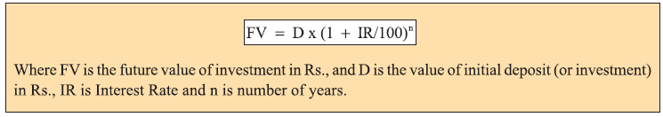
The value of the investment would grow as compound interest is added, until after n years the value of the sum would be:

Example 10.5

The future value of the investment made at present, after 5 years will be:

FV = 22,20,00x 0( 1 + 8/100)^5 = Rs. 32,61,908.40

So in 5 years the initial investment of 22,20,000 will accrue Rs.10,41,908.40 in interest and will be

worth Rs.32,61,908.40. Alternatively, it could equally be said that Rs.32,61908.40 in 5 years time is

worth Rs.22,20,000 now (assuming an annual interest rate of 8%). In other words the present value

of Rs.32,61,908.40 in 5 years time is Rs.22,00,000 now.

The present value of an amount of money at any specified time in the future can be determined by the

following equation.

The net present value method calculates the present value of all the yearly cash flows (1.e. capital costs

and net savings) incurred or accrued throughout the life of a project, and summates them. Costs are represented as a negative value and savings as a positive value. The sum of all the present values is known as the net present value (NPV). The higher the net present value, the more attractive the proposed project.

The present value of a future cash flow can be determined using the equation above. However, it is common practice to use a discount factor (DF) when calculating present value. The discount factor is based on an assumed discount rate (i.e. interest rate) and can be determined by using equation.

The product of a particular cash flow and the discount factor is the present value.

PV = SxDF

The values of various discount factors computed for a range of discount rates (i.e. interest rates) are shown in Table 10.1. The Example 10.6 illustrates the process involved in a net present value analysis.

Example 10.6

Using the net present value analysis technique, let us evaluate the financial merits of the proposed projects shown in the Table below. Assume an annual discount rate of 8% for each project.

Solution

The annual cash flows should be multiplied by the annual discount factors for a rate of 8% to determine the annual present values, as shown in the Table below:

It can be seen that over a 10 year life-span the net present value for Project 1 is Rs.10,254.00, while

for Project 2 it is Rs.10,867.80. Therefore Project 2 is the preferential proposal. The whole credibility of the net present value method depends on a realistic prediction of future interest rates, which can often be unpredictable. It is prudent therefore to set the discount rate slightly above the interest rate at which the capital for the project is borrowed. This will ensure that the overall analysis is slightly pessimistic, thus acting against the inherent uncertain ties in predicting future savings.

Internal rate of return method

It can be seen from Example 10.6 that both projects returned a positive net present value over 10 years, at a discount rate of 8%. However, if the discount rate were reduced there would come a point when the net present value would become zero. It is clear that the discount rate which must be applied, in order to achieve a net present value of zero, will be higher for Project 2 than for Project 1. This means that the average rate of return for Project 2 is higher than for Project 1, with the result that Project 2 is the better proposition.

Example 10.7 illustrates how an internal rate of return analysis is performed.

Example 10.7

A proposed project requires an initial capital investment of Rs.20 000. The cash flows generated by

the project are shown in the table below:

Given the above cash flow data, let us find out the internal rate of return for the project.

Solution

It can clearly be seen that the discount rate which results in the net present value being zero lies

somewhere between 12% and 16%.

For12% discount rate, NPV is positive; for 16% discount rate, NPV is negative. Thus for some discount rate between 12 and 16 percent, present value benefits are equated to present value costs. To find the value exactly, one can interpolate between the two rates as follows:

Thus the internal rate of return for the project is 12.93 %. At first sight both the net present value and

internal rate of return methods look very similar, and in some respects are. Yet there is an important

difference between the two. The net present value method is essentially a comparison tool, which

enables a number of projects to be compared, while the internal rate of return method is designed to

assess whether or not a single project will achieve a target rate of return.

Profitability index

Another technique, which can be used to evaluate the financial viability of projects, is the profitability

index. The profitability index can be defined as:

The application of profitability index is illustrated in Example 10.8.

Example 10.8

Determine the profitability index for the projects outlined in Example 10.6

Project 2 is therefore a better proposal than Project 1.

Factors Affecting Analysis

Although the Examples 10.5 and 10.6 illustrate the basic principles associated with the financial analysis of projects, they do not allow for the following important considerations:

1.The capital value of plant and equipment generally depreciates over time

2.General inflation reduces the value of savings as time progresses. For example, Rs.1000 saved in 1 year’s time will be worth more than Rs.1000 saved in 10 years time.

The capital depreciation of an item of equipment can be considered in terms of its salvage value at the end of the analysis period. The Example 10.9 illustrates the point.

Example 10.9

It is proposed to install a heat recovery equipment in a factory. The capital cost of installing the equipment is Rs.20,000 and after 5 years its salvage value is Rs.1500. If the savings accrued by the heat recovery device are as shown below, we have to find out the net present value after 5 years. Discount rate is assumed to be 8%.

It is evident that over a 5-year life span the net present value of the project is Rs.4489.50. Had the

salvage value of the equipment not been considered, the net present value of the project would have

been only Rs.3468.00.

Real value

Inflation can be defined as the rate of increase in the average price of goods and services. In some countries, inflation is expressed in terms of the retail price index (RPI), which is determined centrally and reflects average inflation over a range of commodities. Because of inflation, the real value of cash flow decreases with time. The real value of sum of money (S) realised in n years time can be determined using the equation.

Where RV is the real value of S realized in n years time. S is the value of cash flow in n years time

and R is the inflation rate (%).

As with the discount factor it is common practice to use an inflation factor when assessing the impact

of inflation on a project. The inflation factor can be determined using the equation.

The product of a particular cash flow and inflation factor is the real value of the cash flow.

The application of inflation factors is considered in Example 10.10.

Example 10.10

Recalculate the net present value of the energy recovery scheme in Example 10.9, assuming the discount rate remains at 8% and that the rate of inflation is 5%.

Solution

Because of inflation; Real interest rate = Discount rate — Rate of inflation

Therefore Real interest rate = 8-5 = 3%

The Example 10.10 shows that when inflation is assumed to be 5%, the net present value of the project reduces from Rs.4489.50 to Rs.4397.88. This is to be expected, because general inflation will always erode the value of future ‘profits’ accrued by a project.

Solved Example:

(i) Two energy conservation projects have been proposed.

For the first project, a capital investment of Rs.1,50,000/- is required and the net annual saving is Rs. 50,000/- for 5 years. The salvage value at the end of 5 years for the first project is Nil. For the second project, a capital investment of Rs. 1,50,000/- yields savings of Rs. 50,000/- for first 2 years each and Rs. 60,000/- for next 3 years each. The salvage value at the end of 5 years for the second project is Rs. 10,000/-. Determine:

a) Net present value for both the projects with a discount factor of 9%.

b) Profitability index for both the projects with a discount factor of 9%.

c) Internal rate of return for both the projects.

(ii) For a VFD retrofit in a compressed air system with an initial investment of Rs.2.55 lakhs the annual savings are Rs.58,000/- The NPV of the project over a six year period for 8% discount rate is Rs.13,134. The NPV of the project over a six year period for 10% discount rate is Rs.(-) 2468 Calculate the exact discount rate for NPV to be zero.

--------------

Chapter 9

Chapter 11